Google ColabでGPU/TPU使用の機械学習

無料でGPUを利用できる機械学習環境Google Colaboratory（以降Google Colab）を試し、とても役に立つと感じたので紹介します。

Google Colabは、Jupyter Notebookと同じような使い勝手で、機械学習に必要なライブラリ等がすでにインストールされているため、ほぼ何の設定もせずにいきなり機械学習のプログラムを実行できます。

さらに、Google Colabのアクセラレータとして使われているNVIDIA Tesla K80というGPUが非常に性能が良いことがわかりました。

また、Google社開発の機械学習に特化したプロセッサTPUも簡単に使うことができました。ただし、本記事ではTPUの性能を十分に引き出す内容までは紹介できていません。

このように素晴らしい機械学習環境が無料で、しかも超簡単に使えることに驚きました。

使用するPC環境は何でもよく、Webブラウザがあれば良いです。本記事ではMac＋Chromeで試しましたが、WindowsやLinuxでも同様にできるはずです。

本記事をなぞることで、準備０の状態から30分〜1時間程度でGoogle Colabでの機械学習を体験することができると思います。

Google Driveの準備
Google Colabの準備
Google Colab実行
まとめ
トラブルシューティング
書籍紹介
参考文献

Google Driveの準備

Google Colabでは、Google Driveをデータ保存領域として使用するため、まずはGoogle Driveの利用開始が必要です。

Google Driveを使ったことがない方はこちらからご自分のGoogle Driveを作成します。（無料の15GBで大丈夫です）

Google Colab作業用のフォルダを”Colab”などのフォルダ名で作成します。

作成したフォルダ名をクリックして「アプリで開く」→「アプリを追加」を選択します。

検索部に”colaboratory”と入力するとColaboratoryが見つかるのでクリックします。

Google DriveのアドオンとしてColaboratoryをインストールします。

以下のようなポップアップが出るので「OK」を押します。

Dialog of confirming connection to google drive

Google Colabの準備

Google Colab起動

上記で作成したGoogle Colab作業用フォルダの「ここにファイルをドロップ」と表示されている部分で右クリック（またはCtrl＋クリック、もしくはタッチパネルを2本指クリック）→「その他」→「Google Colaboratory」をクリックします。

新しくGoogle Colabのタブが立ち上がります。

Google Driveをマウント

Google DriveをGoogle Colabからローカルディスクのように扱えるようにするため、Google Driveをマウントします。

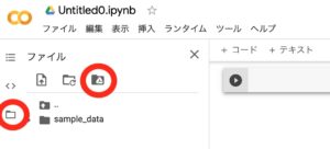
画面左にあるファイルのマークからGoogle Driveマウント（表示されるまでに少し時間がかかります）のアイコンを押します。

以下のポップアップが出るので「GOOGLEドライブに接続」を押します。

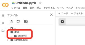
Google Driveをマウントすると以下のようにdrive/My DriveからGoogle Driveが見えるようになります。

以降で使用するサンプルコードとして、こちらからからダウンロードしたwork/mnist_cnn.pyとwork/mnist_cnn_TPU.pyをColabフォルダにアップロードします。

Google Driveのタブに戻り、Colabフォルダを開いている状態の時にファイルをドラッグ＆ドロップするとアップロードでき、以下のように表示されます。

再びGoogle Colabのタブに戻り、コマンド入力部に以下のように打ち込み、Shift＋Enterを押します。

!ls drive/My\ Drive/Colab

頭に!を付けるとサーバマシン上でLinuxコマンドを実行できます。

上記はファイルのリストを表示するlsコマンドの実施例です。

MyとDriveの間に空白があるので、バックスラッシュでエスケープしていますが、'drive/My Drive/Colab'のようにシングルクオートでくくったり、drive/MyDrive/Colabとして空白無しで書いても大丈夫です。

以下のように表示されれば成功です。

Google Colab実行

ここまでで、Google Colabを使う準備ができたので、機械学習のHello World的チュートリアルである手書き文字認識MNISTのコードを使って試していきます。

CPUモード

まずはデフォルトになっているCPUモードで実行します。

使用するPythonコードmnist_cnn.pyの内容は以下です。

'''Trains a simple convnet on the MNIST dataset.

Gets to 99.25% test accuracy after 12 epochs
(there is still a lot of margin for parameter tuning).
16 seconds per epoch on a GRID K520 GPU.
'''

from __future__ import print_function
import tensorflow as tf
from tensorflow.keras.datasets import mnist
from tensorflow.keras.models import Sequential
from tensorflow.keras.layers import Dense, Dropout, Flatten
from tensorflow.keras.layers import Conv2D, MaxPooling2D
from tensorflow.keras import backend as K

batch_size = 128
num_classes = 10
epochs = 12

# input image dimensions
img_rows, img_cols = 28, 28

# the data, split between train and test sets
(x_train, y_train), (x_test, y_test) = mnist.load_data()

if K.image_data_format() == 'channels_first':
    x_train = x_train.reshape(x_train.shape[0], 1, img_rows, img_cols)
    x_test = x_test.reshape(x_test.shape[0], 1, img_rows, img_cols)
    input_shape = (1, img_rows, img_cols)
else:
    x_train = x_train.reshape(x_train.shape[0], img_rows, img_cols, 1)
    x_test = x_test.reshape(x_test.shape[0], img_rows, img_cols, 1)
    input_shape = (img_rows, img_cols, 1)

x_train = x_train.astype('float32')
x_test = x_test.astype('float32')
x_train /= 255
x_test /= 255
print('x_train shape:', x_train.shape)
print(x_train.shape[0], 'train samples')
print(x_test.shape[0], 'test samples')

# convert class vectors to binary class matrices
y_train = tf.keras.utils.to_categorical(y_train, num_classes)
y_test = tf.keras.utils.to_categorical(y_test, num_classes)

model = Sequential()
model.add(Conv2D(32, kernel_size=(3, 3),
                 activation='relu',
                 input_shape=input_shape))
model.add(Conv2D(64, (3, 3), activation='relu'))
model.add(MaxPooling2D(pool_size=(2, 2)))
model.add(Dropout(0.25))
model.add(Flatten())
model.add(Dense(128, activation='relu'))
model.add(Dropout(0.5))
model.add(Dense(num_classes, activation='softmax'))

model.compile(loss=tf.keras.losses.categorical_crossentropy,
              optimizer=tf.keras.optimizers.Adadelta(),
              metrics=['accuracy'])

model.fit(x_train, y_train,
          batch_size=batch_size,
          epochs=epochs,
          verbose=1,
          validation_data=(x_test, y_test))
score = model.evaluate(x_test, y_test, verbose=0)
print('Test loss:', score[0])
print('Test accuracy:', score[1])

以下のコマンドを入力してShift＋Enterを押します。

%%time
%run -i drive/My\ Drive/Colab/mnist_cnn.py

結果は以下でした。はっきり言って手元のPCより遅いです。

Test loss: 0.7461588978767395
Test accuracy: 0.8414000272750854
CPU times: user 52min 42s, sys: 1min, total: 53min 42s
Wall time: 28min 14s

GPUモード

いよいよ本命のGPUモードを使います。
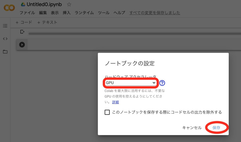
「編集」→「ノートブックの設定」をクリックします。

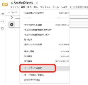
プルダウンからGPUを選択して「保存」を押します。

使用するPythonコードは上記CPUモードで使ったものと同じです。

%%time
%run -i drive/My\ Drive/Colab/mnist_cnn.py

圧倒的に速いです！！！

Test loss: 0.767807126045227
Test accuracy: 0.8345999717712402
CPU times: user 33.2 s, sys: 7.68 s, total: 40.9 s
Wall time: 53.1 s

TPUモード

最後にTPUモードを試します。TPUはGoogle社開発の機械学習に特化したプロセッサ「Tensor Processing Unit」のことです。

「編集」→「ノートブックの設定」と進み、プルダウンからTPUを選択して「保存」を押します。

TPUを使用するためにはPythonコード修正する必要があるので、こちらを参考に手を加えたPythonコードmnist_cnn_TPU.pyの内容は以下です。

'''Trains a simple convnet on the MNIST dataset.

Gets to 99.25% test accuracy after 12 epochs
(there is still a lot of margin for parameter tuning).
16 seconds per epoch on a GRID K520 GPU.
'''

from __future__ import print_function
import tensorflow as tf
from tensorflow.keras.datasets import mnist
from tensorflow.keras.models import Sequential
from tensorflow.keras.layers import Dense, Dropout, Flatten
from tensorflow.keras.layers import Conv2D, MaxPooling2D
from tensorflow.keras import backend as K

batch_size = 128
num_classes = 10
epochs = 12

# input image dimensions
img_rows, img_cols = 28, 28

# the data, split between train and test sets
(x_train, y_train), (x_test, y_test) = mnist.load_data()

if K.image_data_format() == 'channels_first':
    x_train = x_train.reshape(x_train.shape[0], 1, img_rows, img_cols)
    x_test = x_test.reshape(x_test.shape[0], 1, img_rows, img_cols)
    input_shape = (1, img_rows, img_cols)
else:
    x_train = x_train.reshape(x_train.shape[0], img_rows, img_cols, 1)
    x_test = x_test.reshape(x_test.shape[0], img_rows, img_cols, 1)
    input_shape = (img_rows, img_cols, 1)

x_train = x_train.astype('float32')
x_test = x_test.astype('float32')
x_train /= 255
x_test /= 255
print('x_train shape:', x_train.shape)
print(x_train.shape[0], 'train samples')
print(x_test.shape[0], 'test samples')

# convert class vectors to binary class matrices
y_train = tf.keras.utils.to_categorical(y_train, num_classes)
y_test = tf.keras.utils.to_categorical(y_test, num_classes)

# TPU
try:
    tpu = tf.distribute.cluster_resolver.TPUClusterResolver()  # TPU detection
    print('Running on TPU ', tpu.cluster_spec().as_dict()['worker'])
except ValueError:
    raise BaseException('ERROR: Not connected to a TPU runtime; please see the previous cell in this notebook for instructions!')
tf.config.experimental_connect_to_cluster(tpu)
tf.tpu.experimental.initialize_tpu_system(tpu)
strategy = tf.distribute.experimental.TPUStrategy(tpu)
with strategy.scope():

    model = Sequential()
    model.add(Conv2D(32, kernel_size=(3, 3),
                     activation='relu',
                     input_shape=input_shape))
    model.add(Conv2D(64, (3, 3), activation='relu'))
    model.add(MaxPooling2D(pool_size=(2, 2)))
    model.add(Dropout(0.25))
    model.add(Flatten())
    model.add(Dense(128, activation='relu'))
    model.add(Dropout(0.5))
    model.add(Dense(num_classes, activation='softmax'))

    model.compile(loss=tf.keras.losses.categorical_crossentropy,
                  optimizer=tf.keras.optimizers.Adadelta(),
                  metrics=['accuracy'])

    model.fit(x_train, y_train,
              batch_size=batch_size,
              epochs=epochs,
              verbose=1,
              validation_data=(x_test, y_test))
    score = model.evaluate(x_test, y_test, verbose=0)
    print('Test loss:', score[0])
    print('Test accuracy:', score[1])

mnist_cnn.pyに対し、47〜56行目を追加し、57行目以降をwith strategy.scope():の配下にしました。

他のサイトにtf.contrib.〜を使う記述例がありましたが、これはTensorflow 1.x台の記述であり、Google Colabのデフォルト2.xではうまく動かないため、tf.distribute.〜を使用しました。
「ランタイム」→「ランタイムを再起動」でランタイムを再起動し、%tensorflow_version 1.xや%tensorflow_version 2.xとすることでTensorflowバージョンを切り替えられます。

以下のコマンドでTPUを使ったMNISTの学習を実行します。

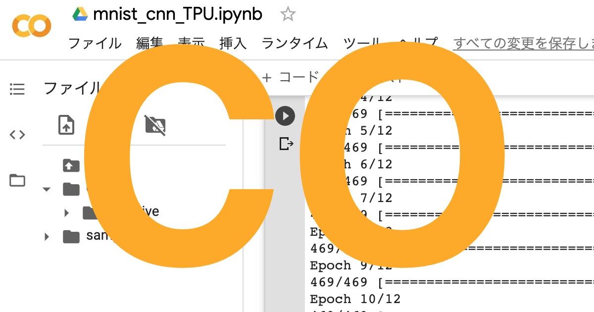
%%time
%run -i drive/My\ Drive/Colab/mnist_cnn_TPU.py

以下のように、今回のMNISTのサンプルではGPUより遅いという結果になりました。

Test loss: 0.7041336297988892
Test accuracy: 0.8344999551773071
CPU times: user 28.8 s, sys: 6.34 s, total: 35.1 s
Wall time: 1min 39s

TPUが得意な対象や学習のさせ方があるようで、こちらで詳しく解説されています。

まとめ

Google ColabでCPU、GPU、TPUでMNISTを使用した機械学習を試し、実時間で比較すると以下のようになりました。

GPU/TPUの効果は絶大ですね。

	CPU	GPU	TPU
Wall Time (s)	1694	53	99

高性能なGPUやTPUを特段のハードルもなく、非常に簡単に使えるため、機械学習を始める方にとって、とても役に立つと思います。

機械学習向け小型マイコンボードJetson-NanoやNVIDIA GPU搭載のMacBookとの速度比較はこちらの記事に書いていますので、ご覧ください。

Google Colabには使用時間やJOBの実行時間に制限がありますが、これから機械学習を始める方には大きな障壁にはならないと思います。
また、このページのように制限内で大規模な学習を実施するための手法もあるようです。

ものづくりに興味があり、いろいろ触り始めたらLinuxの知識が必要になって困っているという方向けに以下のページを作成しましたので、よろしければ参考にしてください。

トラブルシューティング

TPU Name未設定エラー

ノートブックの設定において、TPUを設定していたつもりがNoneになっていた際にこのエラーが出ました。

再度、「編集」→「ノートブックの設定」→「TPU」とすることで解決しました。

ValueError: Please provide a TPU Name to connect to.

書籍紹介

Pythonや画像処理、機械学習関連のおすすめ書籍を紹介します。

人気ブロガーからあげ先生のとにかく楽しいAI自作教室

実践して楽しむことを重視していて、充実のサンプルコードで画像認識やテキスト分析、GAN生成といったAI応用をGoogle Colab環境下で体験できます。

入門 Python 3

基礎から応用までわかりやすい説明でコード例も多数載っていて、初学者の入門書としては必要十分と感じています。

さらにPythonらしいコードの書き方も言及されていて、スマートなコードが書けるようになります。

詳解 OpenCV 3 ―コンピュータビジョンライブラリを使った画像処理・認識

最新のOpenCV4には対応していないのですが、やはりオライリー、基礎を学ぶには十分な情報があり、この本から入ることをおすすめします。

ゼロから作るDeep Learning ―Pythonで学ぶディープラーニングの理論と実装

この本は、機械学習の仕組みを学ぶのにとても良い本だと思います。

Tensorflow/Kerasなどの既存プラットフォームを使うのではなく、基本的な仕組みを丁寧に説明し、かんたんなPythonコードで実装していく手順を紹介してくれます。

機械学習のコードがどのような処理をしているのか、想像できるようになります。

参考文献

Google Drive（https://www.google.com/intl/ja_ALL/drive/using-drive/）
Google Colabの知っておくべき使い方 – Google Colaboratoryのメリット・デメリットや基本操作のまとめ（https://www.codexa.net/how-to-use-google-colaboratory/）
Google ColabのTPUで対GPUの最速に挑戦する（https://qiita.com/koshian2/items/fb989cebe0266d1b32fc）
TPUs in Colab/Enabling and testing the TPU（https://colab.research.google.com/notebooks/tpu.ipynb#scrollTo=FpvUOuC3j27n）
[完全自動接続]Colaboratoryファイルのみで90分・12時間問題を解決した[Selenium使用]（https://qiita.com/shoyaokayama/items/8869b7dda6deff017046）